| timestamp | trade | fill_price | reservation_price | inventory | cash_position | portfolio_value |
|---|---|---|---|---|---|---|
| Loading ITables v2.3.0 from the internet... (need help?) |
Mag7Alpha
https://www.youtube.com/watch?v=GEBxAzIoK8Q&feature=youtu.be
Strategy Overview
Market makers are large financial institutions who act as intermediaries between buyers and sellers. They provide liquidity to traders, taking orders on both sides and reducing the difference between ask and bid price for assets. Market makers make profit from bid ask spreads. Our strategy is market-making on one of the Mag7 stocks, which includes Alphabet, Amazon, Apple, Meta, Microsoft, NVDIA, and Tesla. For our example, we will do MSFT. We will use the Stoikov market-making strategy, so we need two main equations: The first calculates the reservation price based on the equation:
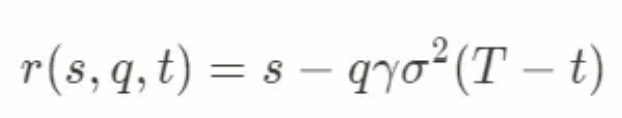
s = current market mid price
q = quantity of assets in inventory of base asset (could be positive/negative for long/short positions)
σ = market volatility
T = closing time, when the measurement period ends (conveniently normalized to 1)
t = current time (T is normalized = 1, so t is a time fraction)
The second sets optimal bid-ask spread using the equation:
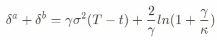
σ = market volatility
T = closing time, when the measurement period ends (conveniently normalized to 1)
t = current time (T is normalized = 1, so t is a time fraction)
δa, δb = bid/ask spread, symmetrical → δa=δb
γ = inventory risk aversion parameter
κ = order book liquidity parameter
Entry conditions: We want to create symmetrical bid and ask orders around the market mid-price, but this could lead to the inventory skewing in one direction if there are significant market movements in one direction. The reference price is where the buy and sell orders will be created around.
After calculating reservation price and optimal bid ask spreads:
Bid offer price = reservation price — optimal spread / 2
Ask offer price = reservation price + optimal spread / 2
We then enter into limit orders on both sides of this quote.
Exit conditions: As the trading day goes on, each parameter of the models will change, and new values for reservation price and optimal spreads will be calculated. We then set new orders based on the new parameters. This cycle continues indefinitely until the end of our backtesting period.
Stop Loss: Instead of setting a specific stop loss, we set inventory limits to try and control the portfolio during momentum shifts. We set this at 15.
Data: We can use ShinyBroker to obtain most of the assets’ attributes, such as price throughout the day, volatility, and timing, via fetch_historical_data.
Blotter:
Ledger:
| timestamp | inventory | cash_position | mid_price | portfolio_value | unrealized_pnl |
|---|---|---|---|---|---|
| Loading ITables v2.3.0 from the internet... (need help?) |
Portfolio Value Over Time
Inventory Level Over Time
Alpha: 1.2683641851897157e-06
Beta: 0.0013455253367804282
benchmark_volatility_annualized: 0.07183856080115263
asset_volatility_annualized: 0.00022642370194626593
benchmark_geometric_mean: 0.9999813518481299
benchmark_arithmetic_mean: -1.8648325749104094e-05
asset_geometric_mean: 1.0000012432731633
asset_arithmetic_mean: 1.2432723904057614e-06
Sharpe Ratio: 0.005490910976717492
Average Return per Trade: 1.2608092485550546
Average Number of Trades per Year: 4357.810344827586